VLOOKUP is a commonly used Excel lookup formula used to retrieve information from adjacent columns of data based on a particular value. For example, imagine if you had a giant list of names and phone numbers in Excel. You could use VLOOKUP to find the name and return the phone number in the next column.
VLOOKUP searches a column for the value selected or mentioned in your VLOOKUP formula. Then, it searches a table or array of data, matches your search value and returns the neighboring value from a corresponding column. Confused? No problem. We’ll explain with some examples in a moment.
The letter V in VLOOKUP stands for “vertical”. It looks for the value in the first column of the given range and returns a value from the same row from another column.
The VLOOKUP function is excellent. However, it is limited to just looking for a single criterion and becomes far more powerful when combined with other formulas like IF and CHOOSE to lookup multiple criteria.
This guide will teach you how to use the VLOOKUP function with multiple criteria and other interesting use cases of the VLOOKUP formula. This guide is applicable for all MS Excel versions.
Table of Contents
- VLOOKUP function
- Syntax
- Parameters
- Example
- VLOOKUP Across Worksheets
- VLOOKUP with an IF Condition
- VLOOKUP with a Helper Column
- VLOOKUP Using the CHOOSE Function
- VLOOKUP with Multiple Criteria
VLOOKUP function
Let’s get started by looking at a basic VLOOKUP. Here, we know one value and using it, we search for a matching value in the same table and return the answer from an adjacent column.
Syntax
VLOOKUP (lookup_value,table_array,colu_index_num,[range_lookup])
Parameters
| Parameters | Explanation |
|---|---|
| lookup_value | This is the value we are searching for in our formula. Once you get the match, VLOOKUP returns a corresponding value from an adjacent column. |
| table_array | This argument takes the cell’s start value and end value of the function’s search. |
| colu_index_num | The value in this argument is how many columns across you want the formula to look and should be a number. |
| range_lookup [Optional] | This argument accepts two values, one is TRUE, and the other is FALSE.
With TRUE, the function returns the closest match. |
Example
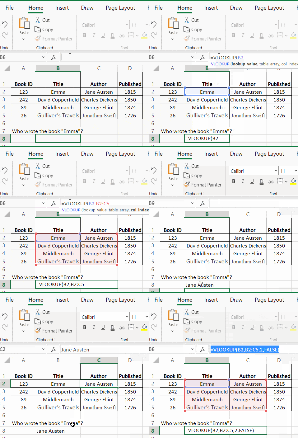
In the example below, we find the author of the book “Emma”. The known value is the book title, and we will use this to find its author.
Enter the formula in cell B8 or any other cell you wish the answer displayed.
=VLOOKUP(B2, B2:C5,2 FALSE).
Let’s break down each parameter in the formula and understand what it means. First, B2 contains the known data, which is the book’s title, the lookup_value.
B2:C5 is the table_array where the answer is in one of the cells. The third parameter is “2”, which denotes the column index from where we’ll draw our answer. The column index is the number of columns to the right of the lookup_value that we want to return. Our table_array starts with column B, so B is column 1, and column 2 is C.
The fourth parameter is FALSE, which returns an exact match for the formula.
VLOOKUP Across Worksheets
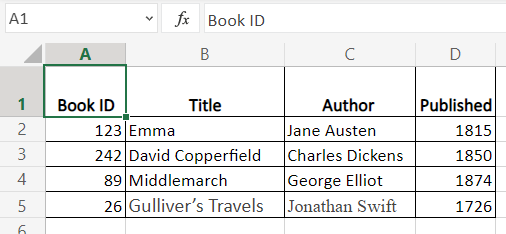
Now, let’s look at an example of using VLOOKUP to look up values across worksheets. For instance, we have a worksheet named Books, containing book publishing details.
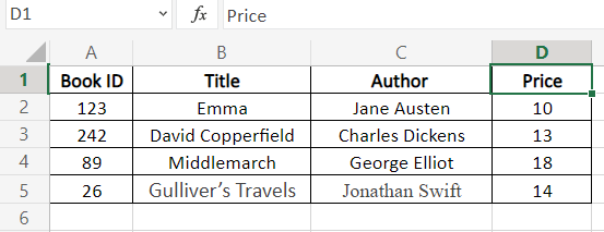
There’s another worksheet named Price, which contains the price of various books.
As you can see from the example above, we can use VLOOKUP to lookup values from another worksheet.
We have the book’s details such as the Book ID, Title, Author, and Published year in the ‘Book’ worksheet. Likewise, the worksheet ‘Price’ contains the details such as Book ID, Title, Author, and Price.
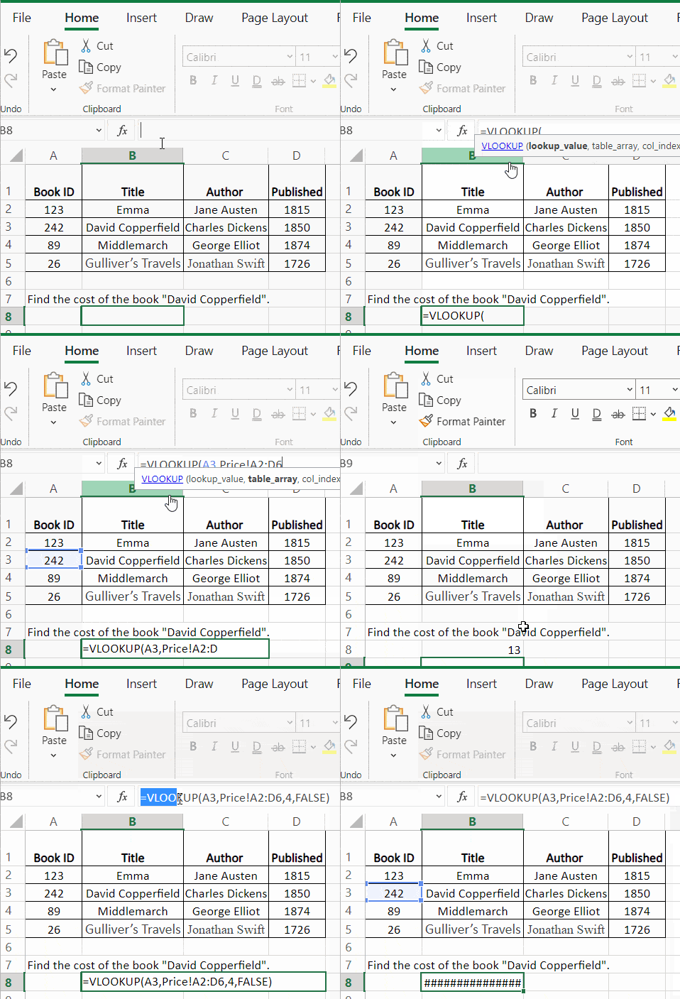
To know the price of the book “David Copperfield”, and use the formula
=VLOOKUP(A3, Price!A2:D6,4, FALSE)
Cell A3 in the worksheet Book contains Book ID 242.
The second argument Price!A2:D6 specifies the table_array. Price is the other worksheet’s name which contains the details about the price of the books.
It refers to the cells A2:D6. From there, the formula finds a match in column A, counts four columns across and returns the price as 13.
Here’s another example of VLOOKUP in action:
VLOOKUP with Multiple Criteria
So VLOOKUP is pretty handy. But what if we need VLOOKUP to take into account multiple criteria? Using our examples so far, what if we want it to match an author ID and an author and then return a result? VLOOKUP by itself can’t handle multiple criteria.
However, combine VLOOKUP with some other functions, and it can handle multiple criteria. These are the different ways to do it.
- VLOOKUP with IF condition.
- VLOOKUP with HELPER column.
- VLOOKUP using CHOOSE function.
VLOOKUP with an IF condition
You can combine IF conditions with the VLOOKUP function to check complex criteria and return a True/False or Yes/No value.
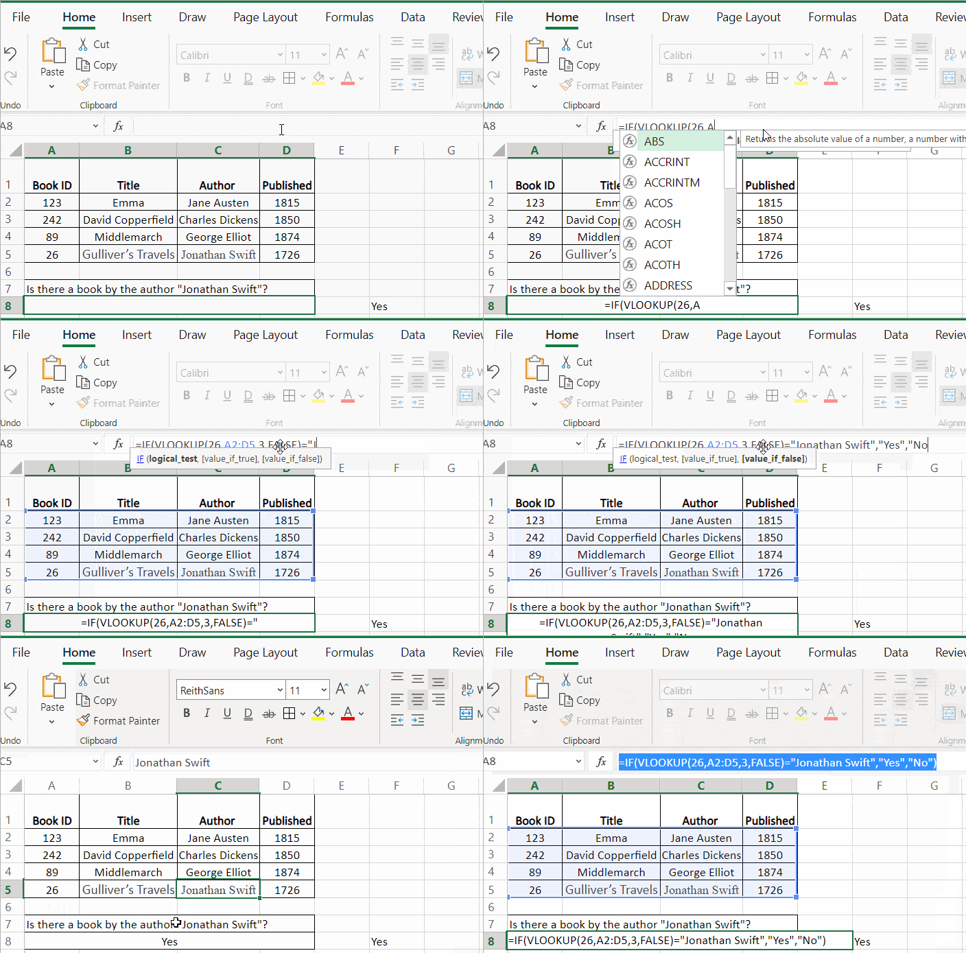
In the following example, we find the author for book ID “26”. We then check if it matches a particular name, in this case, “Jonathan Swift”, using a combination of IF and VLOOKUP.
To achieve this, we nest our VLOOKUP in an IF statement:
=IF(VLOOKUP(26, A2:D5, 3, FALSE)=” Jonathan Swift”, “Yes”, “No”)
VLOOKUP with a Helper Column
A helper column adds an extra column to the given data to simplify specific calculations.
You can use it to help the VLOOKUP function identify multiple criteria.
Let’s consider the worksheet “Book”, where we wish to get the year of publication based on a book title and author.
The book title and author are separate in columns B and C. As VLOOKUP cannot match two columns, we can instead combine (or concatenate) columns C and D and create a new column. In this case, column D is our helper column.
Use the formula =B2&”-” &C2 or simply B2&C2 to concatenate the values in the two columns.
The “&” concatenates the data in the two cells, and the “-” act as separators.
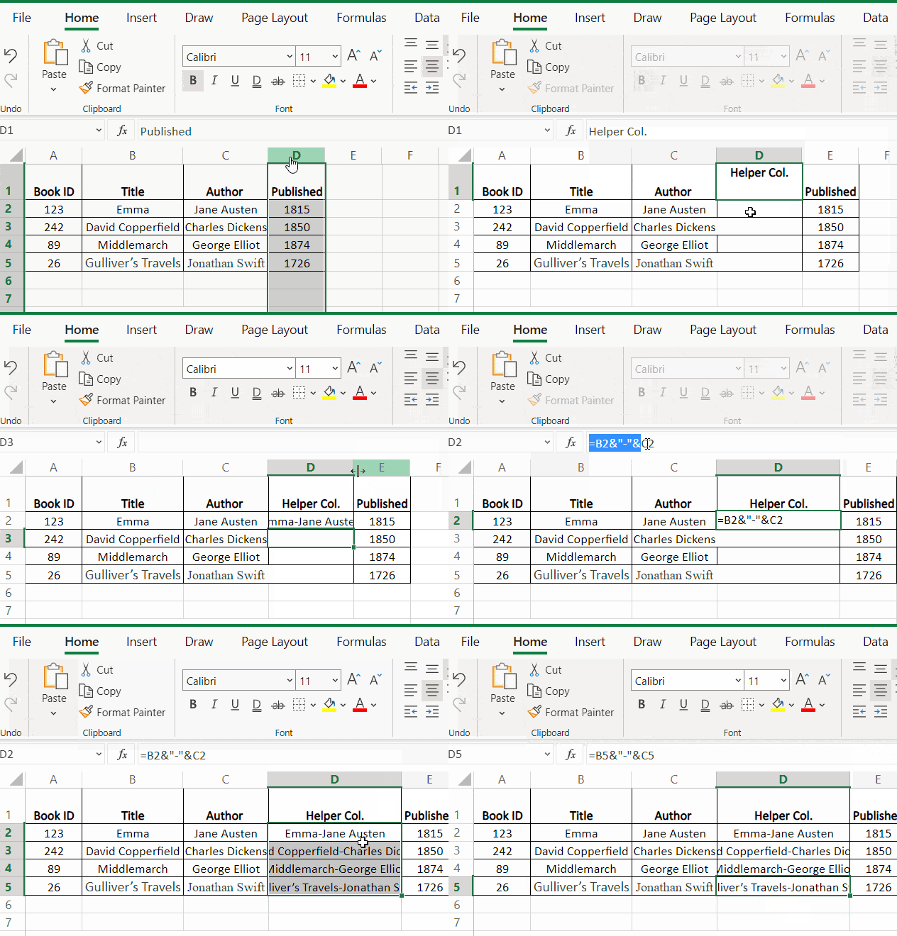
Drag the formula down to copy it to the respective cells below.

Now we have our helper column ready to use in our VLOOKUP.
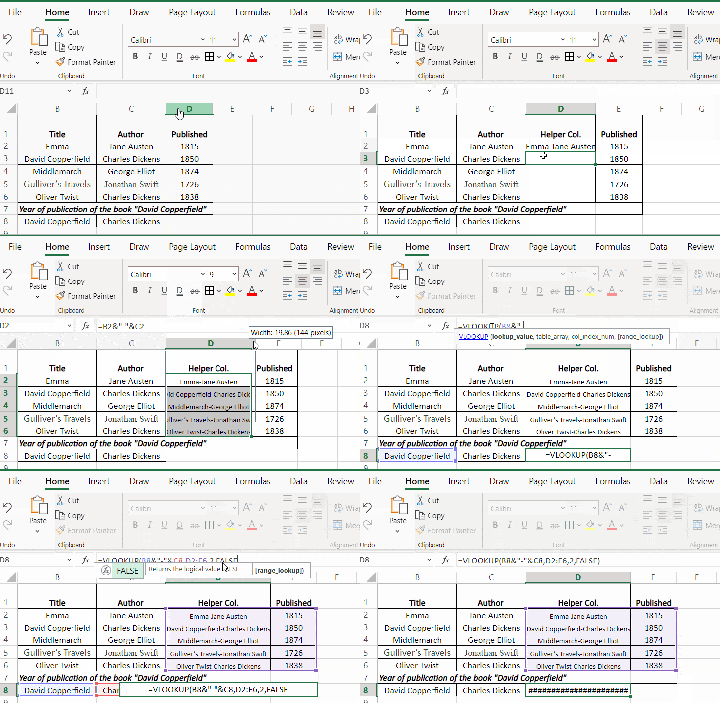
In this example, cells B8 and C8 contain the criteria, column D has the concatenated values, and column E has the result.
Mention the column index as “2” as it is the second column from the helper column, which contains the matching value.
And FALSE returns us an exact match. Therefore, the result appears in D8 as 1850.
VLOOKUP Using the CHOOSE Function
You can use the CHOOSE function to return a value from a list based on the position that we set WITHIN a VLOOKUP formula.
So in this instance, we are nesting the CHOOSE function within our VLOOKUP formula.
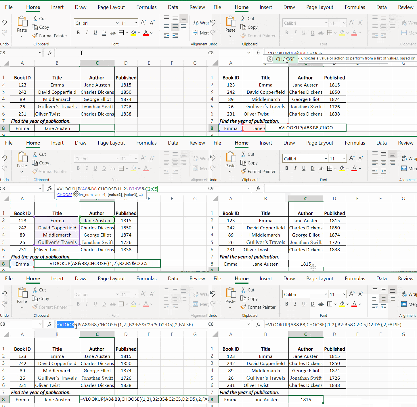
In this example, to find the year of publication, we use the formula:
=VLOOKUP(A8&B8, CHOOSE({1,2}, B2:B5&C2:C5, D2:D5),2, FALSE).
Notice that the two lookup arguments, A8 and B8, are concatenated by & symbol.
A8 has the book name “Emma”, and B8 has the author name “Jane Austen”.
The list to choose from is specified as {1,2}. It identifies the next column in the same row. In a similar way to a helper column, by using CHOOSE, we make use of a list {1,2}.
The next argument in the formula is B2:B5&C2:C5, D2:D5. This concatenates the values in columns B and C and pulls the result from column D.
The value 2 represents that D is the second column from the list, and FALSE returns an exact match.
We get the result 1815 in cell C8.
Frequently Asked Questions
1.What is the difference between VLOOKUP and XLOOKUP?
- The main drawback of VLOOKUP is that it could search vertically. If you want to search horizontally in rows (top to bottom), you need to switch to HLOOKUP. XLOOKUP, on the other hand, can handle both vertical and horizontal lookups.
- A VLOOKUP can only search from left to right. If the value we are looking for is to the left of the given range, then VLOOKUP won’t work. XLOOKUP can search both left and right of the lookup_value in the given range of cells.
- XLOOKUP has additional parameters such as what to display if the lookup value doesn’t exist. Additionally, with XLOOKUP, you can explicitly set whether to search from first to last or reverse order.
- The major drawback of XLOOKUP is that it is only available on the more recent versions of Microsoft Office!
2. What are the types of matches a VLOOKUP function can do?
- Exact match – Use FALSE in the fourth parameter in the VLOOKUP function to get the exact match
- Approximate match – Use TRUE in the fourth parameter in the VLOOKUP function to get
- Wildcard match – VLOOKUP supports wildcard characters to make a partial match.
Final Thoughts
In this article, we’ve looked at how to do a basic VLOOKUP and combine VLOOKUP with other functions to lookup a result based on multiple criteria.
If you’re looking at what to learn next, we recommend learning how to use the XLOOKUP function, or if you are on Excel 2019 or older, INDEX MATCH.


